Cities

miles_graph() returns an undirected graph over the 128 US cities from the datafile miles_dat.txt. The cities each have location and population data. The edges are labeled with the distance between the two cities.

This example is described in Section 1.1 in Knuth’s book (see [1] and [2]).

References.

[1]	Donald E. Knuth, “The Stanford GraphBase: A Platform for Combinatorial Computing”, ACM Press, New York, 1993.

[2]	http://www-cs-faculty.stanford.edu/~knuth/sgb.html

Out:

Loaded miles_dat.txt containing 128 cities.
digraph has 128 nodes with 8128 edges
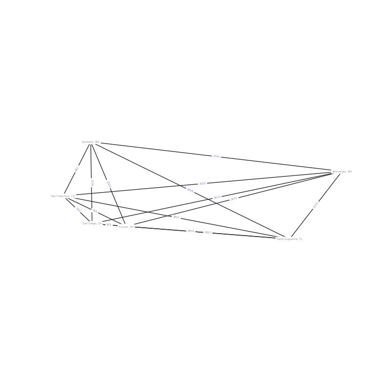
Subgraph has 6 nodes with 15 edges
['San Diego, CA', 'San Francisco, CA', 'Worcester, MA', 'Spokane, WA', 'Tucson, AZ', 'Saint Augustine, FL']

# Based on example from NetworkX

import re
import sys

import matplotlib.pyplot as plt
import networkx as nx
import grave


def miles_graph():
    """ Return the cites example graph in miles_dat.txt
        from the Stanford GraphBase.
    """
    # open file miles_dat.txt.gz (or miles_dat.txt)
    import gzip
    fh = gzip.open('knuth_miles.txt.gz', 'r')

    G = nx.Graph()
    G.position = {}
    G.population = {}

    cities = []
    for line in fh.readlines():
        line = line.decode()
        if line.startswith("*"):  # skip comments
            continue

        numfind = re.compile("^\d+")

        if numfind.match(line):  # this line is distances
            dist = line.split()
            for d in dist:
                G.add_edge(city, cities[i], weight=int(d))
                i = i + 1
        else:  # this line is a city, position, population
            i = 1
            (city, coordpop) = line.split("[")
            cities.insert(0, city)
            (coord, pop) = coordpop.split("]")
            (y, x) = coord.split(",")

            G.add_node(city)
            # assign position - flip x axis for matplotlib, shift origin
            G.position[city] = (-int(x) + 7500, int(y) - 3000)
            G.population[city] = float(pop) / 1000.0
    return G


if __name__ == '__main__':

    G = miles_graph()

    print("Loaded miles_dat.txt containing 128 cities.")
    print("digraph has %d nodes with %d edges"
          % (nx.number_of_nodes(G), nx.number_of_edges(G)))
    cities = ['San Diego, CA',
              'San Francisco, CA',
              'Saint Augustine, FL',
              'Spokane, WA',
              'Worcester, MA',
              'Tucson, AZ']

    # make subgraph of cities
    H = G.subgraph(cities)
    print("Subgraph has %d nodes with %d edges" % (len(H), H.size()))
    print(H.nodes)

    # draw with grave
    plt.figure(figsize=(8, 8))
    # create attribute for label
    nx.set_edge_attributes(H,
                           {e: G.edges[e]['weight'] for e in H.edges},
                           'label')

    # create stylers
    def transfer_G_layout(network):
        return {n: G.position[n] for n in network}

    def elabel_base_style(attr):
        return {'font_size': 4,
                'font_weight': .1,
                'font_family': 'sans-serif',
                'font_color': 'b',
                'rotate': True,  # TODO: make rotation less granular
                }

    elabel_style = grave.style_merger(grave.use_attributes('label'),
                                      elabel_base_style)

    grave.plot_network(H, transfer_G_layout,
                       node_style=dict(node_size=20),
                       edge_label_style=elabel_style,
                       node_label_style={})

    # scale the axes equally
    plt.xlim(-5000, 500)
    plt.ylim(-2000, 3500)

    plt.show()

Total running time of the script: ( 0 minutes 0.081 seconds)